- 公開日:
スプレッドシートで複数条件の条件付き書式を設定する方法
Google スプレッドシートで条件付き書式を設定している場合、違った条件でもセルの色が変わるなどの設定ができれば、よりフレキシブルで見やすいシートが作成できます。
スプレッドシートでは、特定のセルや行といった範囲に複数の条件付き書式を設定することができます。
例えば、数値が100以上だと黄、200以上だと青、文字列が変更で赤のように、シートへの入力状況によって条件が次々に発動します。
この記事では、スプレッドシートで複数の条件付き書式を同範囲に設定する方法を詳しく紹介します。
スプレッドシートで複数条件の条件付き書式を設定する方法
Google スプレッドシートでは、特定の範囲やセルに複数の条件付き書式を設定したり、条件付き書式の設定内に複数のセルを条件とすることができます。
複数の条件付き書式を設定する場合、複数の条件のうちどの条件を優先するかを設定することで、柔軟な変更が可能となります。
複数のセルを条件とする場合は、AND関数をカスタム数式で設定します。
以下より、スプレッドシートで複数の条件付き書式を設定する方法と、複数のセルを条件とする方法を分けて詳しく解説します。
複数の条件付き書式を設定する
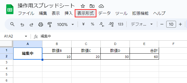
「表示形式」をクリックします。
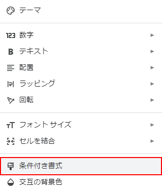
「条件付き書式」を選択します。
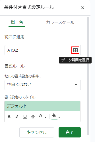
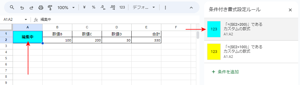
右側に条件付き書式設定ルールが表示されます。
「データ範囲を選択」をクリックします。
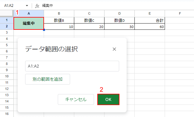
「データ範囲の選択」が表示されます。
①範囲を選択し、②「OK」ボタンをクリックします。
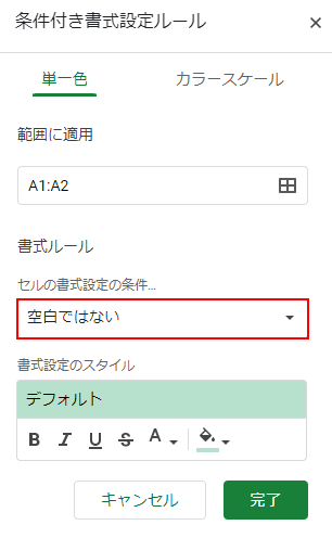
「セルの書式設定の条件…」をクリックします。

「カスタム数式」を選択します。
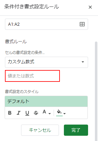
「値または数式」をクリックします。
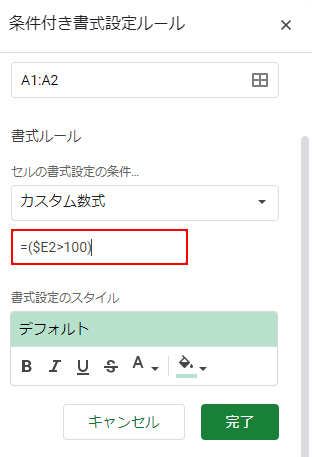
「=($E2>100)」と入力します。
これは「もしE2の値が100より大きかったら」を意味します。
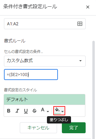
「塗りつぶし」をクリックします。
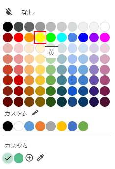
色(例:黄)を選択します。
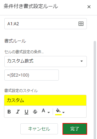
「完了」ボタンをクリックします。
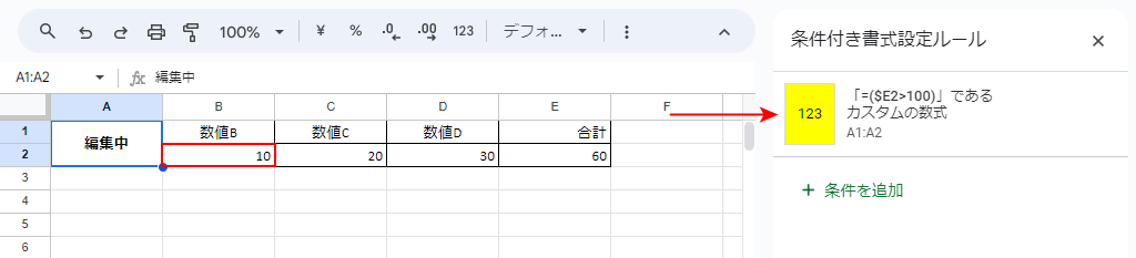
条件付き書式が設定されました。
E2の合計値が100より上になるように、B2の数値を変更します。
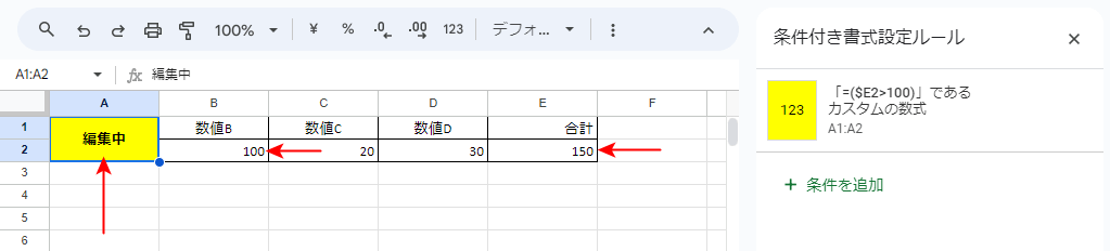
B2の数値を変更したため、E2の合計値が100より大きくなりました。
セルの色が変わりました。
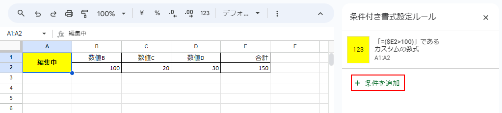
「条件を追加」をクリックします。
同様の範囲に適応されています。
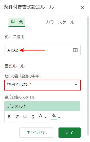
「セルの書式設定の条件…」をクリックします。
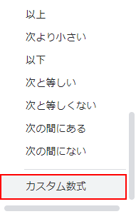
「カスタム数式」を選択します。
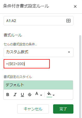
「=($E2>200)」と入力します。
これは「もしE2の値が200より大きかったら」を意味します。
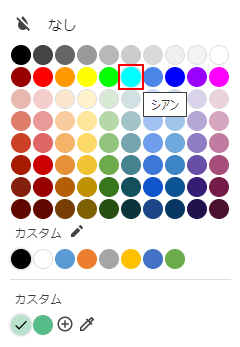
「塗りつぶし」で色(例:シアン)を選択します。
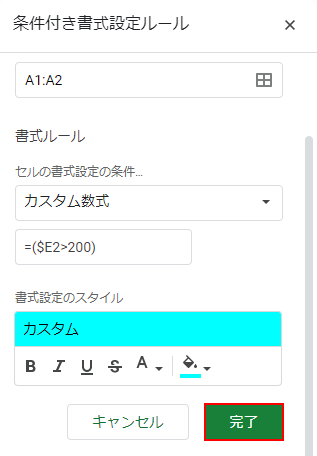
「完了」ボタンをクリックします。
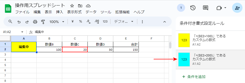
新たに条件付き書式が設定されました。
E2の合計値が200より上になるように、C2の数値を変更します。
C2の数値を変更したため、E2の合計値が200より大きくなりました。
しかし、優先順位が低いためセルの色が変わりません。
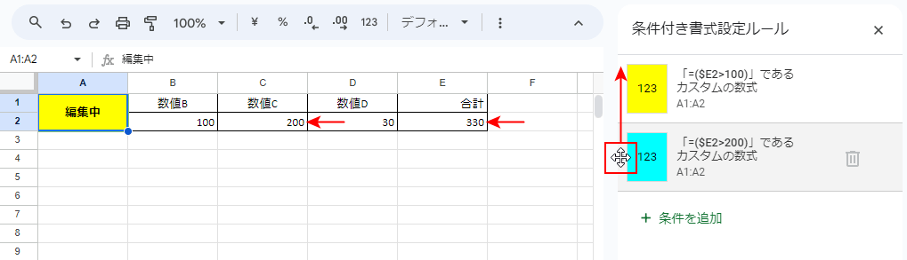
優先順位を上位にするため、追加した条件の左側にカーソルを合わせ、十字矢印にマウスポインタが変わったら、上方向にドラッグします。
優先順位が最上位となり、セルの色が変わりました。
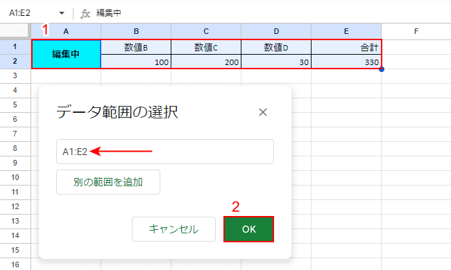
条件を追加し、①先ほど設定したセルを含む範囲を選択し、②「OK」ボタンをクリックします。
選択した範囲が自動的に入力されています。
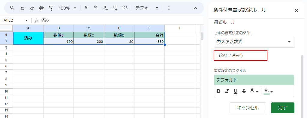
「カスタム数式」に「=($A1="済み")」と入力します。
これは「もしA1セルに〈済み〉と入力されたら」を意味します。
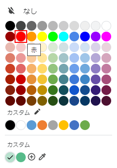
「塗りつぶし」で色(例:赤)を選択します。
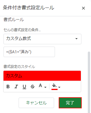
「完了」ボタンをクリックします。
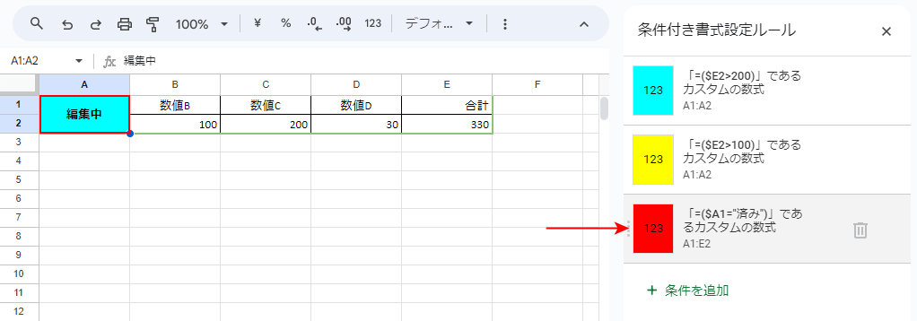
新たに条件付き書式が設定されました。
A1セルに「済み」と入力します。
A1に済みと入力したため、別条件とは重複しないセルの色が変わりました。
しかし、重複しているセルは優先順位が低いため、セルの色が変わりません。
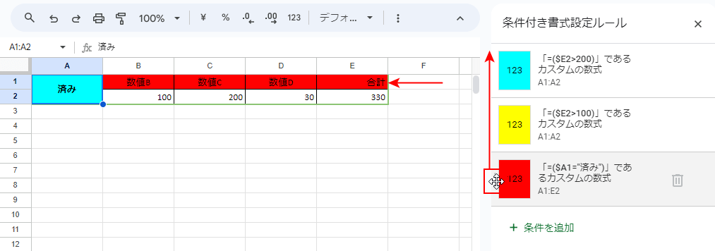
優先順位を上位にします。
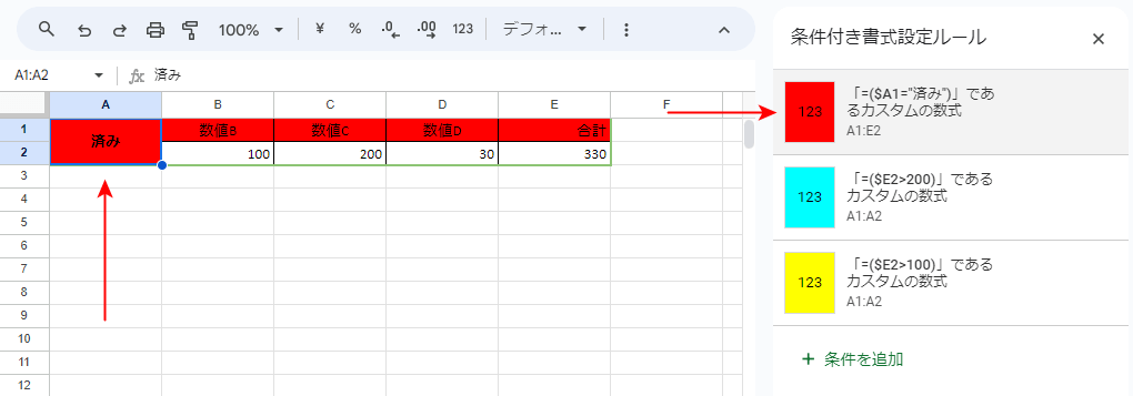
優先順位が最上位となり、セルの色が変わりました。
これで複数の条件付き書式を設定することができました。
このシートでは、A1とA2のセルが結合されているため、列での条件判定の結果、B2からE2のセルの色が変わってません。
スプレッドシートで条件付き書式を設定する際は、このような性質があることに注意が必要です。
列における条件付き書式の性質については、以下の記事にある「列全体に対する数式が作用している」で詳しく解説しています。
複数のセルを条件付き書式で条件とする
Google スプレッドシートで、複数のセルを条件付き書式で条件とする場合、AND関数をカスタム数式で設定します。
以下の記事にある「複数のセルをチェックで行の色を変更する」で、詳しく解説しています。