- 公開日:
スプレッドシートで作るシフト表カレンダー
スプレッドシートを使ってシフト表カレンダーを作成することで、効率的で簡単にシフトを管理することが可能です。
従来の手書きや単純な表計算ソフトよりも使いやすく、柔軟性があります。
この記事では、スプレッドシートを使ったシフト表カレンダーについて解説します。
スプレッドシートで作るシフト表カレンダー
スプレッドシートを使ったシフト表カレンダーについてご紹介します。
今回は例として、2024年5月のシフト表を作成していきます。
![基準日を設定する](https://g-tips.jp/wp-content/uploads/create-shift-schedule-calendar-in-spreadsheet1.png)
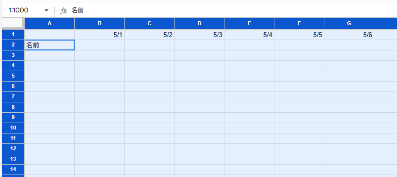
①氏名の見出しを入力(例:A2セル)します。
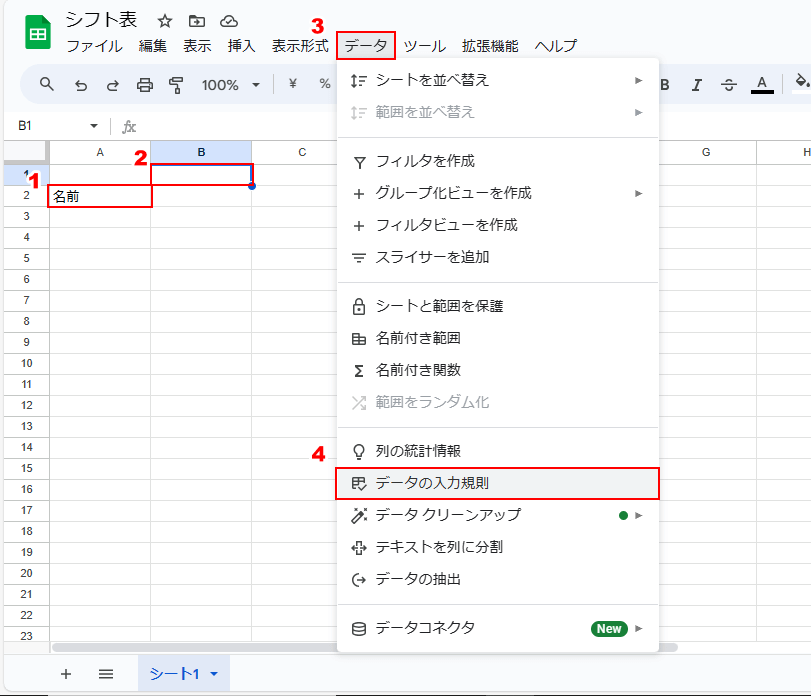
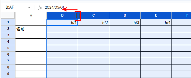
次に日付を入力する行の先頭(B1セル)に基準日を設定します。
②基準日を入力するセルを選択し、③メニューバーの「データ」をクリックし、③「データの入力規則」をクリックします。
![ルールを追加をクリックする](https://g-tips.jp/wp-content/uploads/create-shift-schedule-calendar-in-spreadsheet27.png)
「ルールを追加」をクリックします。
![有効な日付を選択する](https://g-tips.jp/wp-content/uploads/create-shift-schedule-calendar-in-spreadsheet28.png)
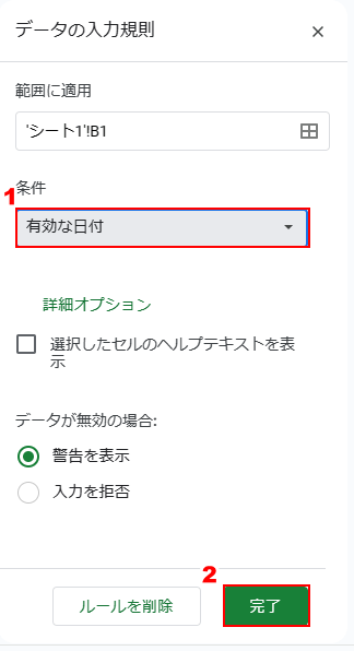
①条件に「有効な日付」を選択し、②「完了」ボタンをクリックします。
![基準日を決定する](https://g-tips.jp/wp-content/uploads/create-shift-schedule-calendar-in-spreadsheet29.png)
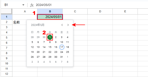
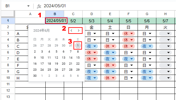
①基準日を設定するセルをダブルクリックすると、カレンダーが表示されるので、②基準日の日付(例:2024年5月1日)を選択します。
カレンダー右上部に表示されている左右の山括弧マークをクリックすることで、月の変更が可能です。
![基準日の隣のセルに数式を入力する](https://g-tips.jp/wp-content/uploads/create-shift-schedule-calendar-in-spreadsheet2.png)
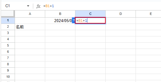
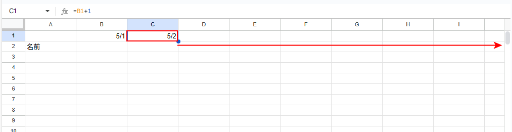
基準日の隣のセル(例:C1セル)に「=B1+1」と入力します。
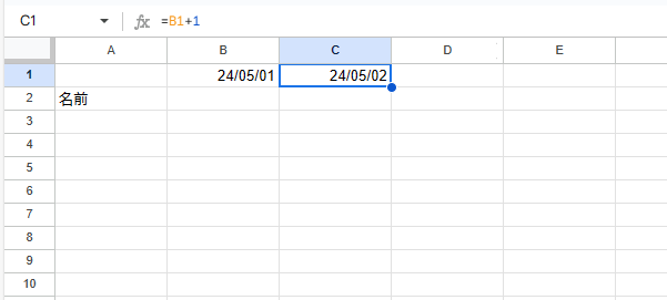
![基準日の翌日の日付が表示された](https://g-tips.jp/wp-content/uploads/create-shift-schedule-calendar-in-spreadsheet33.png)
基準日の翌日の日付が表示されました。
![表示形式を変更する](https://g-tips.jp/wp-content/uploads/create-shift-schedule-calendar-in-spreadsheet30-1.png)
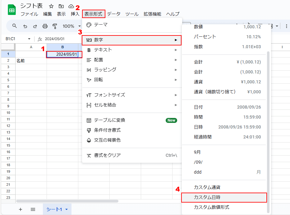
①基準日と翌日の日付が表示されているセル(例:B1セルとC1セル)をドラッグで選択し、②「表示形式」、③「数字」、④「カスタム日時」の順にクリックします。
![「月」または「日」をクリックする](https://g-tips.jp/wp-content/uploads/create-shift-schedule-calendar-in-spreadsheet38.png)
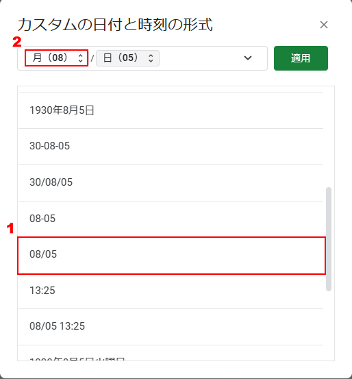
①お好みの表示形式を選択(例:08/05)します。
数字の先頭の「0」を消したい場合は、②「月」または「日」をクリックします。
![「千行ゼロなしの月」をクリックする](https://g-tips.jp/wp-content/uploads/create-shift-schedule-calendar-in-spreadsheet32.png)
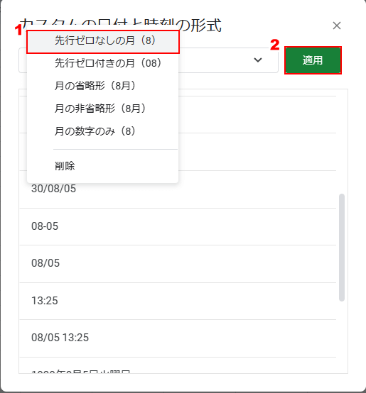
表示された項目の中から、①「先行ゼロなしの月」を選択し、②「適用」ボタンをクリックします。
![Z列まで指定する](https://g-tips.jp/wp-content/uploads/create-shift-schedule-calendar-in-spreadsheet34.png)
表示形式が変更されました。
次に数式を入力したセル(例:C1セル)を選択し、右下の四隅の点をクリックしたまま、Z列までドラッグします。
![Z列からU列までドラッグし指定する](https://g-tips.jp/wp-content/uploads/create-shift-schedule-calendar-in-spreadsheet3.png)
Z列まで連続した日付が自動入力されます。
日数が足りないので、列を増やしていきます。
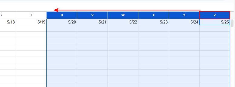
Z列の先頭(ローマ字が表示されている場所)をクリックしたまま、U列までドラッグします。
このドラッグで指定した分だけ、列を増やすことが出来ます。
今回は、5月末日まで6日分足りないので、Z列から6列指定しています。
![Z列から右に6列セルを挿入する](https://g-tips.jp/wp-content/uploads/create-shift-schedule-calendar-in-spreadsheet4.png)
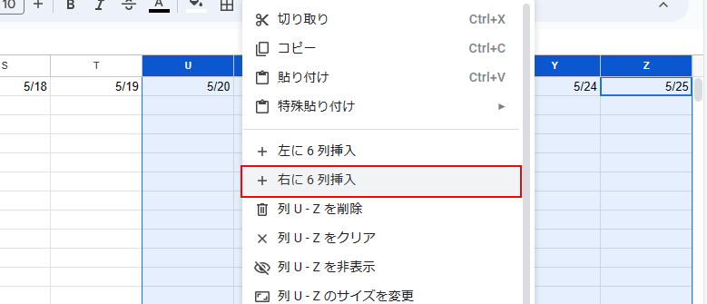
指定したセル上で右クリックを押し、表示されたメニューの中の「右に6列挿入」をクリックします。
![AA列からAFセルまで日付を入力する](https://g-tips.jp/wp-content/uploads/create-shift-schedule-calendar-in-spreadsheet5.png)
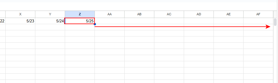
最後の日付が表示されているセル(例:Z1セル)を選択し、右下の四隅の点をクリックしたまま最後の列までドラッグします。
![一か月分の日付が入力できた](https://g-tips.jp/wp-content/uploads/create-shift-schedule-calendar-in-spreadsheet6.png)
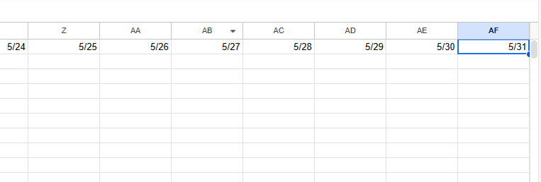
これで表示する月の、1か月分の日付が入力できました。
![セル全体を指定する](https://g-tips.jp/wp-content/uploads/create-shift-schedule-calendar-in-spreadsheet7.png)
次に、表に枠を挿入します。
セル全体を指定します(A2セル上で「Ctrl」キーを押したまま、「A」キーを押すと全体が指定されます)。
![枠線を挿入する](https://g-tips.jp/wp-content/uploads/create-shift-schedule-calendar-in-spreadsheet8.png)
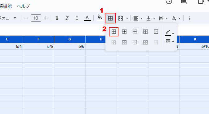
①メニューバーの「枠線」をクリックし、②「全ての枠線」をクリックします。
これですべてのセルに枠線が挿入されます。
![日付が表示されている列を指定する](https://g-tips.jp/wp-content/uploads/create-shift-schedule-calendar-in-spreadsheet9.png)
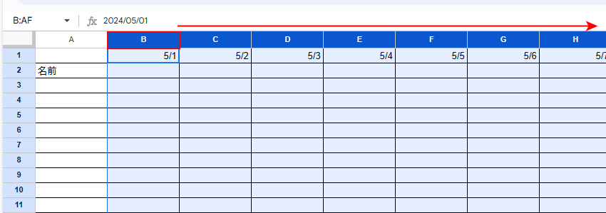
日付が表示されている列を指定(B列からAF列)し、セルの幅を調整します。
![列幅を調整する](https://g-tips.jp/wp-content/uploads/create-shift-schedule-calendar-in-spreadsheet10.png)
列と列の間にマウスポイントを合わせて、クリックしたまま左に動かし列幅を調整します。
![日付の先頭の下のセルに数式を入力する](https://g-tips.jp/wp-content/uploads/create-shift-schedule-calendar-in-spreadsheet12-1.png)
次に、日付の下に曜日を入力していきます。
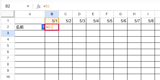
日付の先頭の下のセル(例:B2セル)に「=B1」と入力します。
直接、曜日を入力しても構いませんが、数式を使用することで指定した「月」の日付に連動させるようにしていきます。
![B2セルからAF2セルまでドラッグする](https://g-tips.jp/wp-content/uploads/create-shift-schedule-calendar-in-spreadsheet13.png)
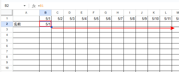
B2セルを選択し、右下の四隅の点をクリックしたまま、日付が入力されている最後の列までドラッグします。
![メニューからカスタム日時を開く](https://g-tips.jp/wp-content/uploads/create-shift-schedule-calendar-in-spreadsheet15.png)
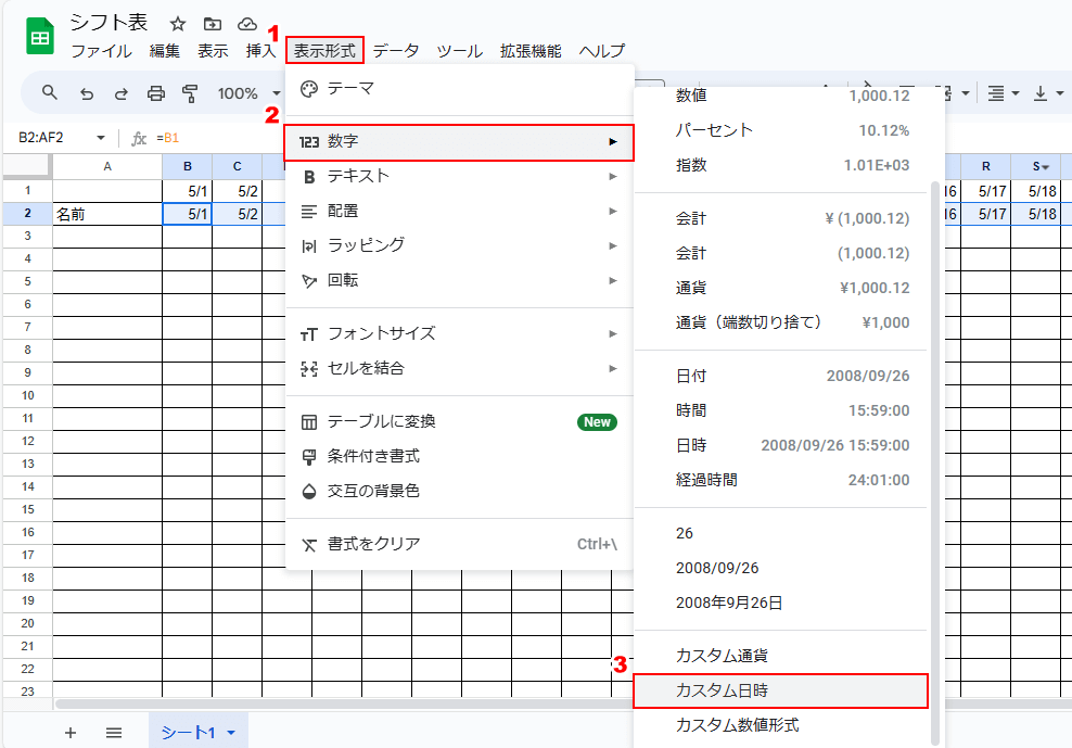
曜日のセルが指定されたままの状態で、①メニューバーの「表示形式」②「数字」③「カスタム日時」の順にクリックします。
![表示形式を選択する](https://g-tips.jp/wp-content/uploads/create-shift-schedule-calendar-in-spreadsheet16.png)
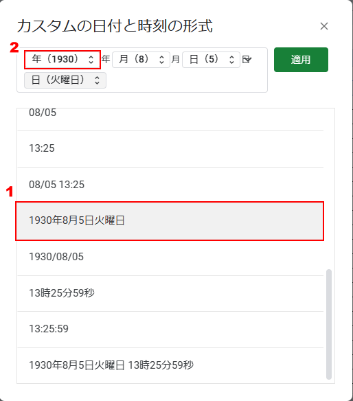
①曜日が表示される項目を選択し、②曜日以外の項目(例:年)をクリックします。
![項目を削除する](https://g-tips.jp/wp-content/uploads/create-shift-schedule-calendar-in-spreadsheet17.png)
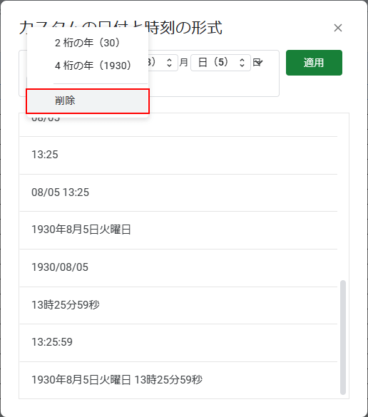
表示された項目の中の「削除」をクリックします。
「月」「日」も同様に削除しましょう。
![適用ボタンを押す](https://g-tips.jp/wp-content/uploads/create-shift-schedule-calendar-in-spreadsheet18.png)
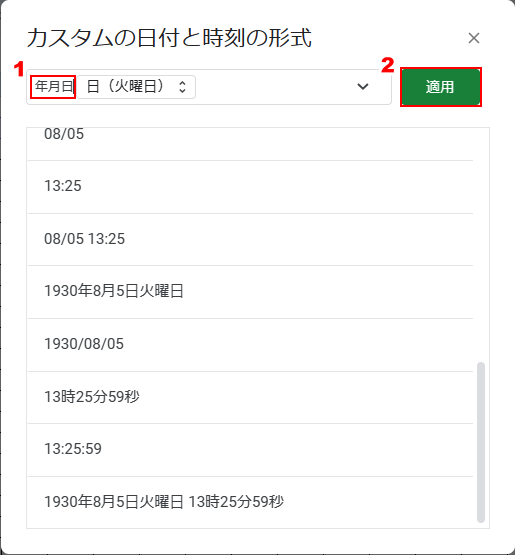
①表示されている余分な文字、記号を削除し、②「適用」ボタンをクリックします。
![曜日の表記に変更できた](https://g-tips.jp/wp-content/uploads/create-shift-schedule-calendar-in-spreadsheet19.png)
曜日の表記に変更できました。
![メニューからカスタム数値形式を開く](https://g-tips.jp/wp-content/uploads/create-shift-schedule-calendar-in-spreadsheet20.png)
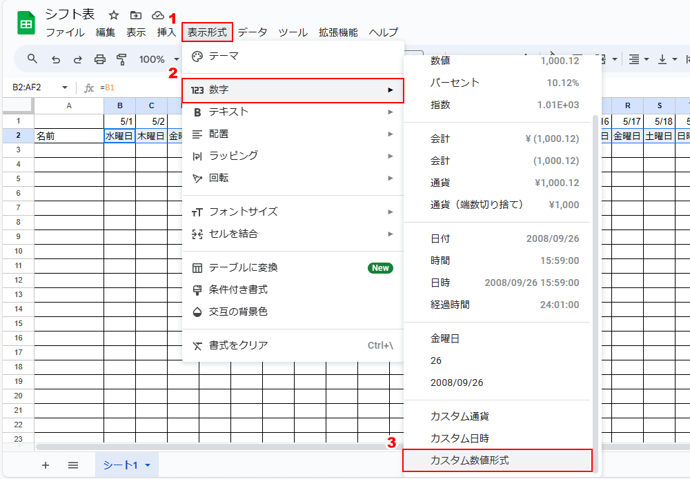
「月」「火」「水」などの表記にする場合は、①「表示形式」、②「数字」、③「カスタム数値形式」の順でクリックします。
![dddと入力する](https://g-tips.jp/wp-content/uploads/create-shift-schedule-calendar-in-spreadsheet21.png)
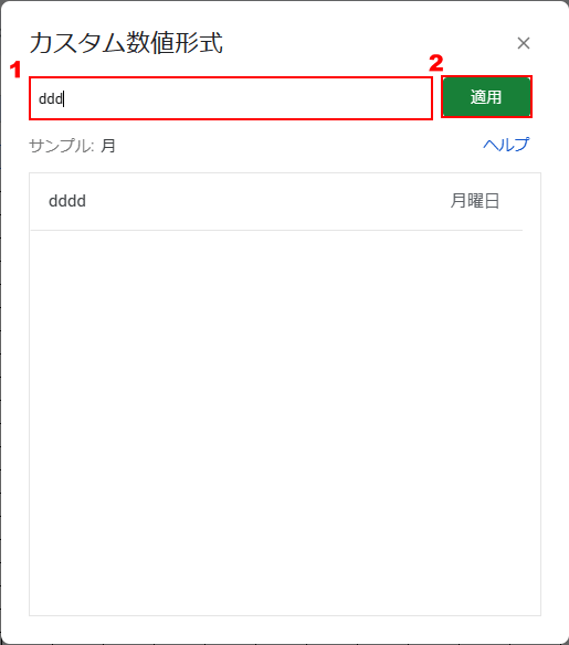
①カスタム数値形式の入力欄に「ddd」と入力し、②「適用」ボタンをクリックします。
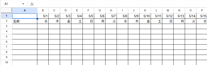
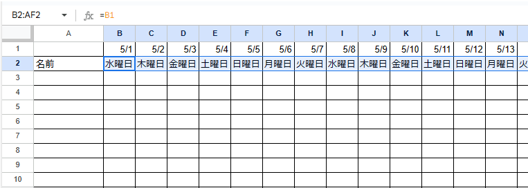
![曜日の表示形式が変更された](https://g-tips.jp/wp-content/uploads/create-shift-schedule-calendar-in-spreadsheet22-1.png)
曜日の表示形式が変更されました。
![プルダウンを設定した](https://g-tips.jp/wp-content/uploads/create-shift-schedule-calendar-in-spreadsheet25.png)
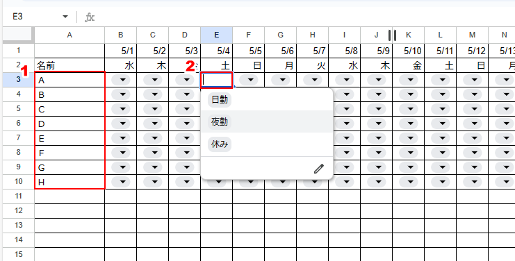
①シフト表に記載する氏名(例:A、B、C等)を入力し、②セルにプルダウン(例:日勤、夜勤、休み)を設定します。
プルダウンを設定することで、シフト入力を簡単に行うことが出来ます。
プルダウンの設定方法については、下記の記事にて詳しく解説していますので、ぜひご参照ください。
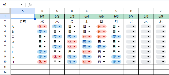
![シフト表が完成した](https://g-tips.jp/wp-content/uploads/create-shift-schedule-calendar-in-spreadsheet35.png)
シフト表が完成しました。
色の設定や、細かなセルや列の幅などを調整して、仕上げましょう。
![表示する月を変更する](https://g-tips.jp/wp-content/uploads/create-shift-schedule-calendar-in-spreadsheet39.png)
「月」を変更してみましょう。
①基準日を設定したセルをダブルクリックし、②カレンダーの月を変更、③表示させる月の1日をクリックします。
![日付が変更され曜日も変更された](https://g-tips.jp/wp-content/uploads/create-shift-schedule-calendar-in-spreadsheet37.png)
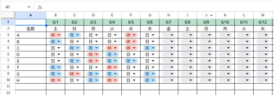
日付が変更され、曜日も連動して表示されました。