- 公開日:
スプレッドシートの条件付き書式で列全体を塗りつぶす方法
Google スプレッドシートでは条件付き書式を用いることで、特定のセルが条件を満たした時に、列全体の色が変わり、一目でシートの状態が分かるような設定を行うことができます。
この記事では、スプレッドシートの条件付き書式で列全体を塗りつぶすことに焦点を当て、分かりやすく紹介します。
スプレッドシートの条件付き書式で列全体を塗りつぶす方法
Google スプレッドシートでは条件付き書式を用いて、列全体を一括で塗りつぶす際、「カスタム数式」を設定して列全体の色を塗りつぶすことはできません。
列全体に対して条件を設定しても、列上にあるセルと隣り合うセル(同行のセル)の条件を対象としてしまうためです。
「カスタム数式」以外の条件においては、列全体を塗りつぶすことは可能です。
空白のセルを条件とする場合
列全体のセルが空白である場合に、塗りつぶす方法は以下の通りです。
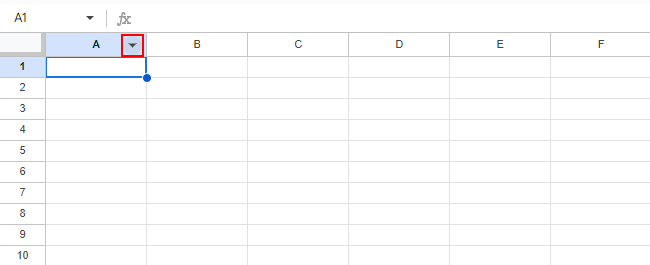
設定する列にある逆三角形をクリックします。
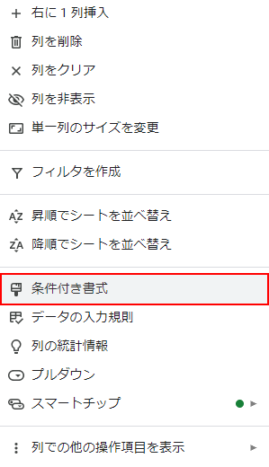
「条件付き書式」を選択します。
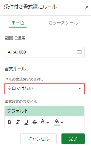
「セルの書式設定の条件」をクリックします。
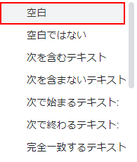
「空白」を選択します。
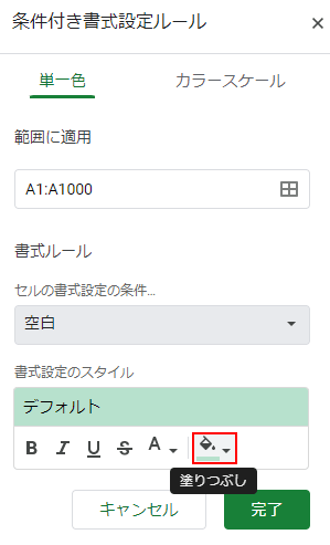
「塗りつぶし」をクリックします。
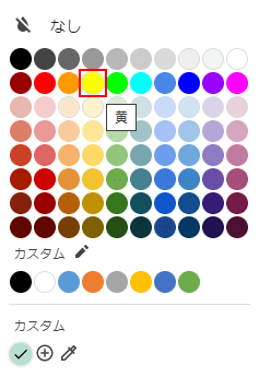
塗りつぶされる色(例:黄)を選択します。
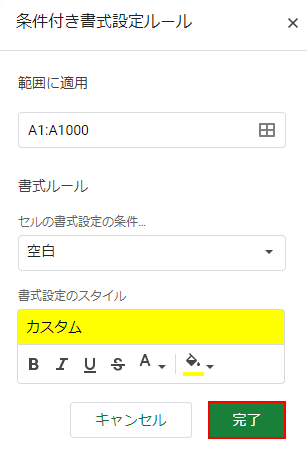
「完了」ボタンをクリックします。
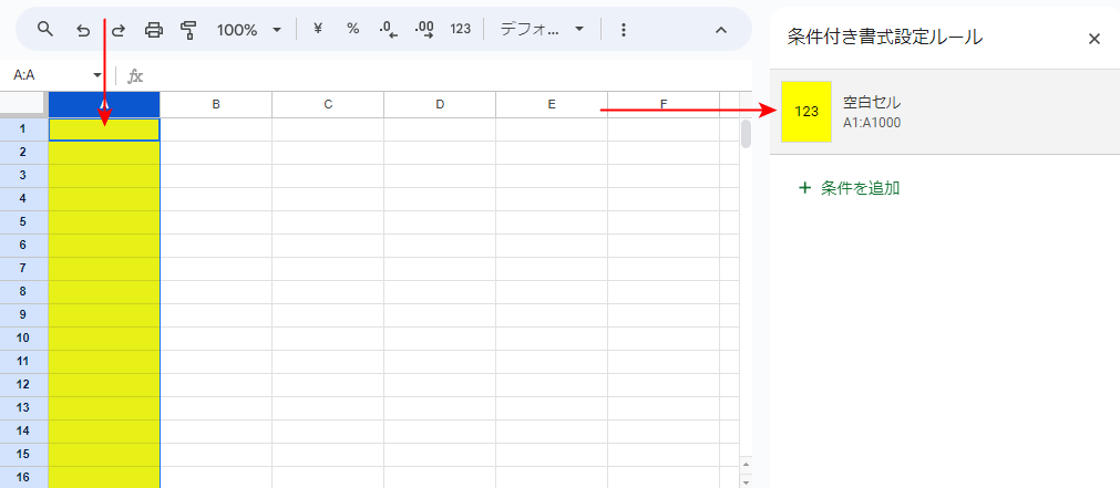
条件付き書式設定ルールが追加され、列全体が塗りつぶされました。
次を含むテキストを条件とする場合
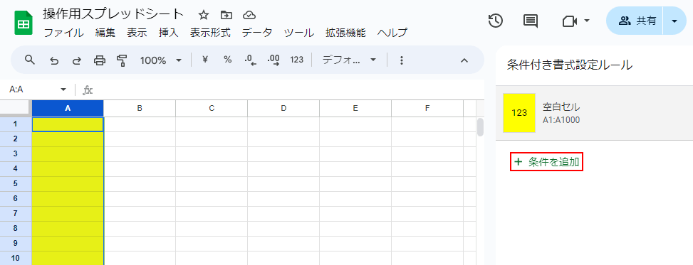
「条件を追加」をクリックします。
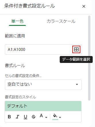
「データ範囲を選択」をクリックします。
「データ範囲の選択」が表示されます。
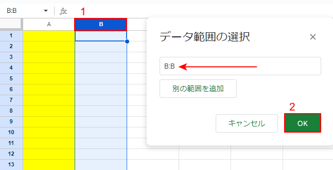
①塗りつぶしたい列をクリックし、②「OK」ボタンをクリックします。
ここでは、B列を選択したので、B:Bと自動的に入力されました。
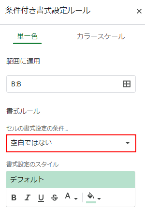
「セルの書式設定の条件…」をクリックします。
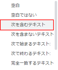
「次を含むテキスト」を選択します。
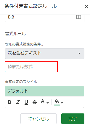
「値または数式」をクリックします。
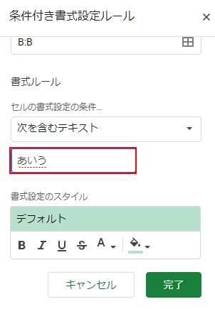
条件としたい文字列(例:あいう)を入力します。
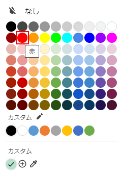
「塗りつぶし」で塗りつぶされる色(例:赤)を選択します。
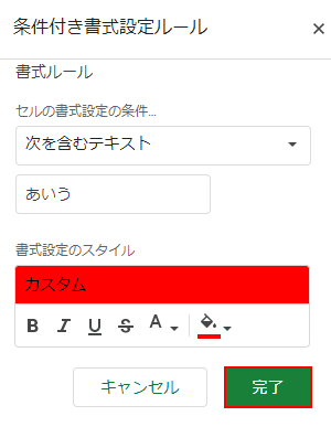
「完了」ボタンをクリックします。
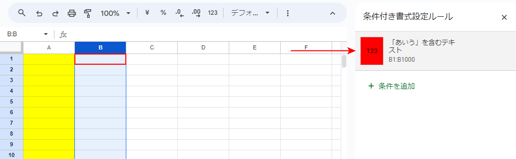
条件付き書式設定ルールが追加されました。
条件とした列のセルを選択します。
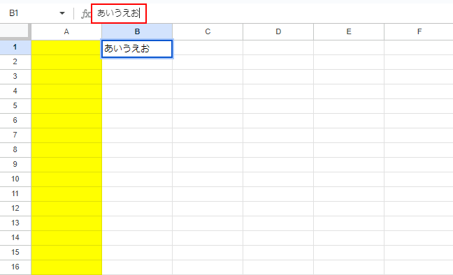
条件を含んだ文字列(例:あいうえお)を入力します。
入力したセルを選択します。
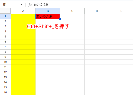
Ctrl+Shift+↓を押します。列の最後のセルまで選択します。
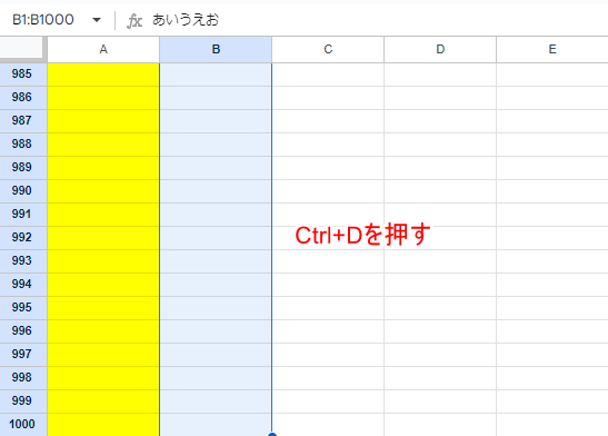
Ctrl+Dを押します。
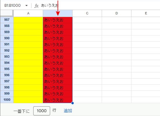
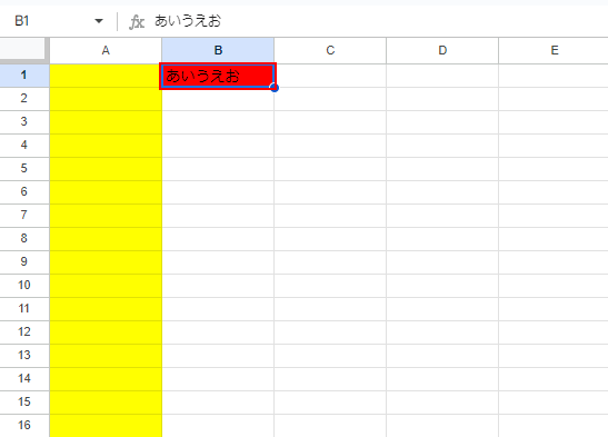
列全体にテキストが入力され、塗りつぶすことができました。
次より小さいを条件とする場合
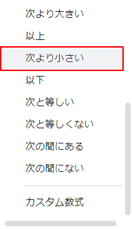
「データ範囲の選択」でC列を選択し、「セルの書式設定の条件…」で「次より小さい」を選択します。
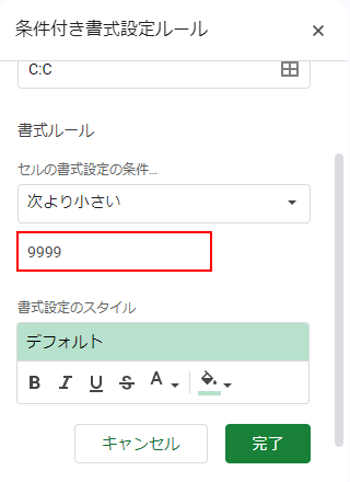
「値または数式」に条件としたい数値(例:9999)を入力します。
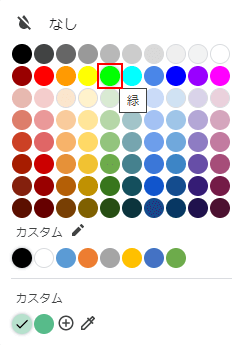
塗りつぶされる色(例:緑)を選択します。
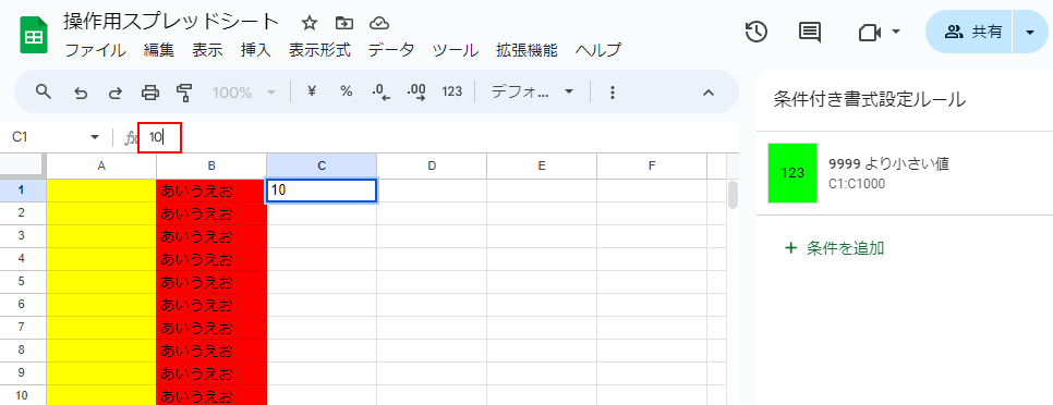
条件付き書式のルールを追加できたら、条件に当てはまる数値(例:10)を入力します。
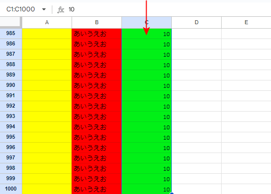
上記「次を含むテキストを条件とする場合」と同様にセルをコピーします。
列全体に数値が入力され、塗りつぶすことができました。
スプレッドシートの条件付き書式で色がつかない場合
Google スプレッドシートで上記のような操作をしても色がつかない場合、様々な事が要因として考えられます。
以下の記事にて、スプレッドシートの条件付き書式で色がつかない場合の対処法を詳しく紹介しています。