- 公開日:
スプレッドシートの条件付き書式で行全体を塗りつぶす方法
Google スプレッドシートを複数人で共有して使用している際、特定のセルが条件を満たした時に、行の色が変わり、一目でシートの状態が分かるような設定にすることができます。
例えば、特定の文字が入力されたり、数値が〇〇以上になったりなど、様々な条件を元に行の色を変えられれば、業務の進捗やシートの入力作業確認などが効率的に進められます。
この記事では、スプレッドシートの条件付き書式機能を用いて、行全体を塗りつぶす方法を分かりやすく紹介します。
スプレッドシートの条件付き書式で行全体を塗りつぶす方法
Google スプレッドシートの条件付き書式を用いて、行全体を塗りつぶす場合、条件付き書式でカスタム数式を入力します。
以下より、様々な条件におけるカスタム数式を入力して、行全体を塗りつぶす、言い換えれば、色を変更する方法を詳しく解説します。
特定の文字列を条件にする場合
特定のセルに、決められた文字列が入力された際に、行を塗りつぶす方法は以下の通りです。
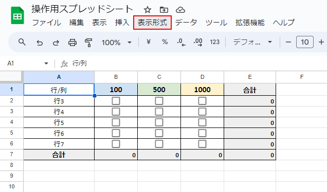
「表示形式」をクリックします。
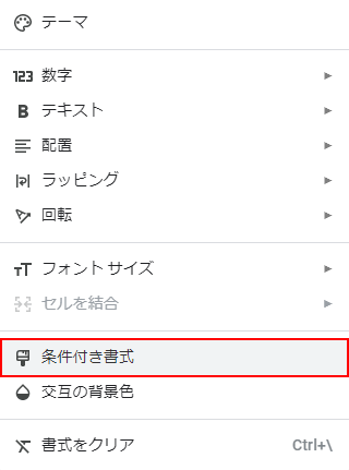
「条件付き書式」を選択します。
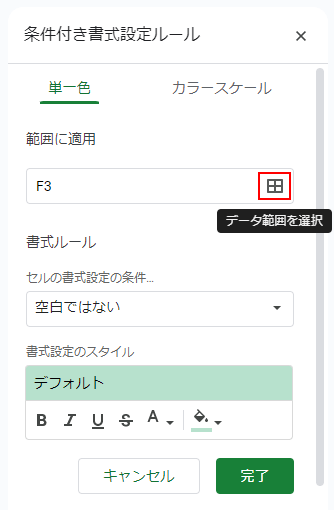
右側に「条件付き書式設定ルール」が表示されます。
「データ範囲を選択」をクリックします。
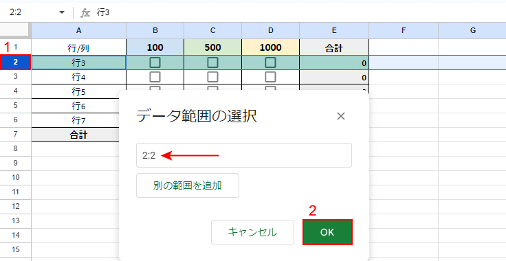
「データ範囲の選択」ダイアログボックスが表示されます。
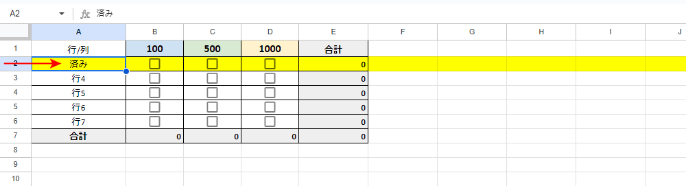
①塗りつぶしたい行をクリックし、②「OK」ボタンをクリックします。
2行目を選択したので、2:2と自動的に入力されました。
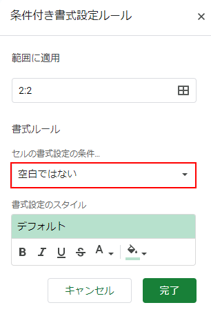
「セルの書式設定の条件…」をクリックします。
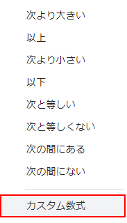
「カスタム数式」を選択します。
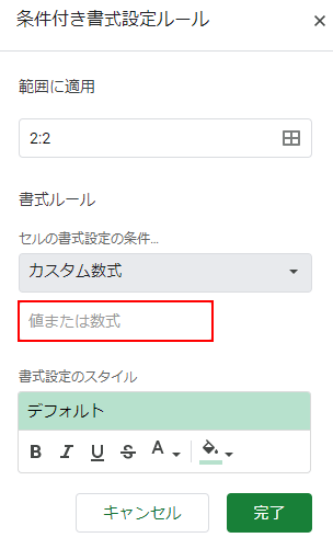
「値または数式」をクリックします。
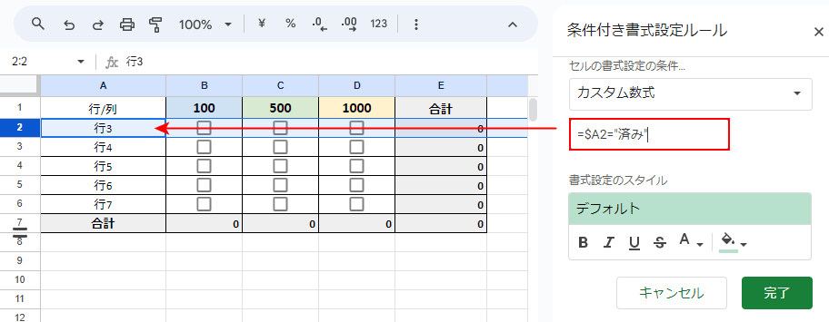
「=$A2="済み"」と入力します。
これは、A2セルに「済み」と入力されたことが条件ということを意味します。
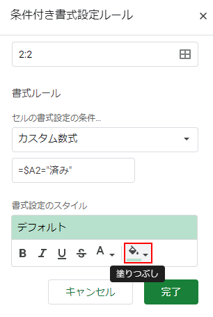
「塗りつぶし」をクリックします。
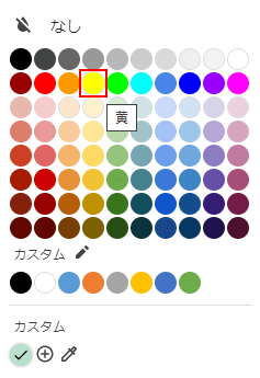
塗りつぶされる色(例:黄)を選択します。
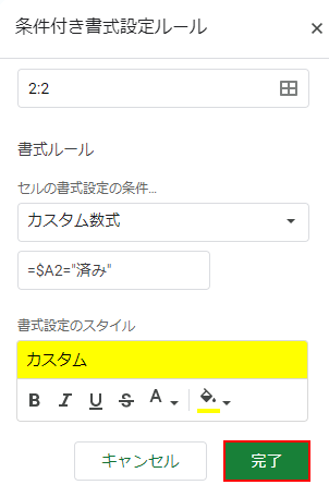
「完了」ボタンをクリックします。
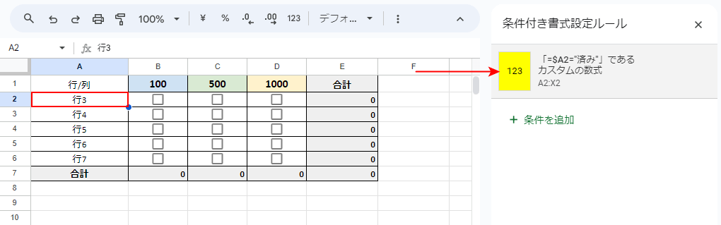
条件付き書式設定ルールが追加されました。
条件としたA2セルを選択します。
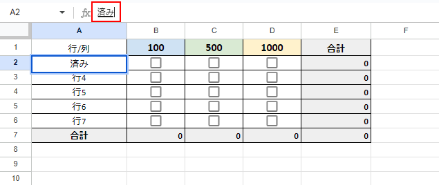
条件とした文字列「済み」と入力します。
行全体が塗りつぶされました。
数値の大きさを条件にする場合
特定のセルに決められた数値が入力された際に、行を塗りつぶす方法は以下の通りです。
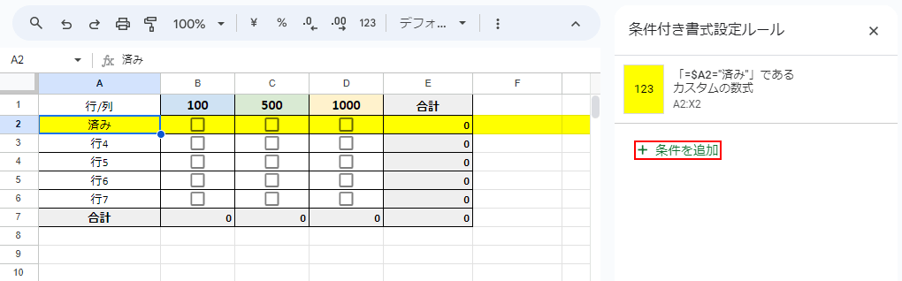
「条件を追加」をクリックします。
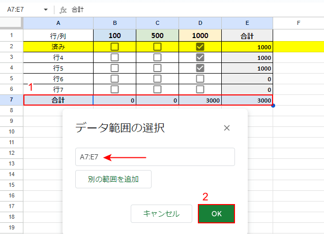
今回は入力されている行全体を塗りつぶすことにします。
①範囲を選択して、②「OK」ボタンをクリックします。

「カスタム数式」を選択し、「値または数式」に「=$E7>4000」と入力します。
これは、E7セルが4000より大きい数値となることが条件ということを意味します。
4000より小さい数値の場合は「=$E7<4000」、決められた数値の場合は「=$E7=4000」と入力します。
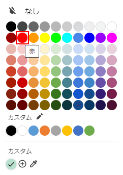
「塗りつぶし」で塗りつぶされる色(例:赤)を選択します。
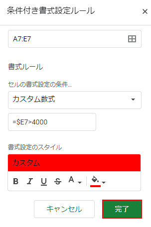
「完了」ボタンをクリックします。
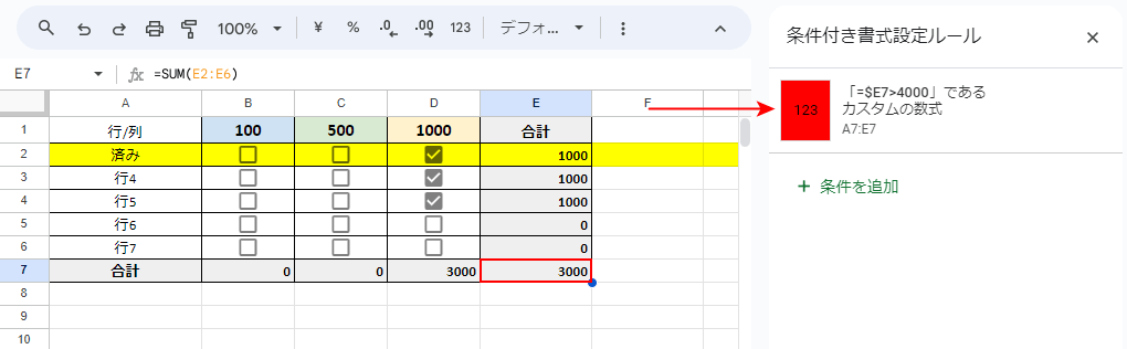
条件付き書式設定ルールが追加されました。
条件としたE7セルの数値を変更します。
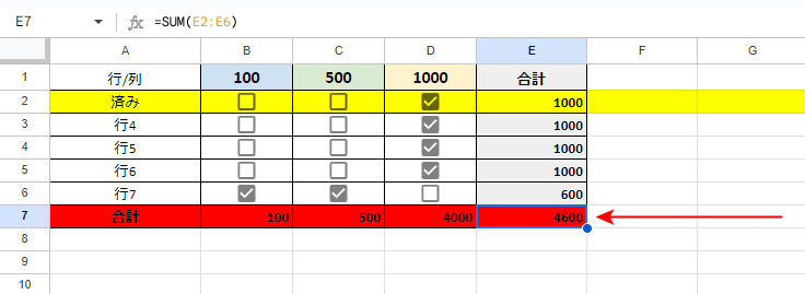
4000より大きい数値となったので、行全体が塗りつぶされました。
チェックボックスのチェックを条件にする場合
特定のチェックボックスがチェックされたことを条件に、行を塗りつぶすことができます。
複数のチェックボックスや、いずれかのチェックボックスという条件も含め、以下の記事にて詳しく紹介しています。
スプレッドシートの条件付き書式で色がつかない場合
Google スプレッドシートで、上記のような操作をしても色がつかない場合、様々な事が要因として考えられます。
以下の記事にて、スプレッドシートの条件付き書式で色がつかない場合の対処法を詳しく紹介しています。