- 公開日:
スプレッドシートの条件付き書式で別シートを参照する方法
Google スプレッドシートでは、関数を利用することによって、別のシートを参照して、条件付き書式を設定することが可能です。
この記事では、スプレッドシートにおける条件付き書式の条件を、別シートから参照する方法を分かりやすく紹介します。
スプレッドシートの条件付き書式で別シートを参照する方法
Google スプレッドシートで別シートから参照して条件付き書式を設定する場合、INDIRECT関数を使用します。
INDIRECT関数とは、指定されたセルの入力内容を返す関数です。INDIRECT関数を利用して、別シートのセルを指定し、その内容に応じた条件を設定します。
以下より、スプレッドシートの条件付き書式で、INDIRECT関数をカスタム数式で利用し、別シートの内容を条件とする方法を詳しく解説します。
別シートの特定のセルを条件とする
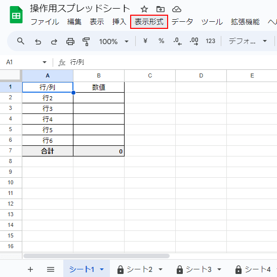
「表示形式」をクリックします。
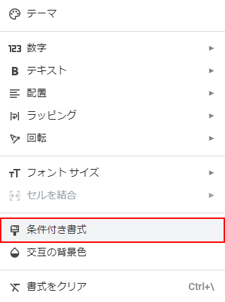
「条件付き書式」を選択します。
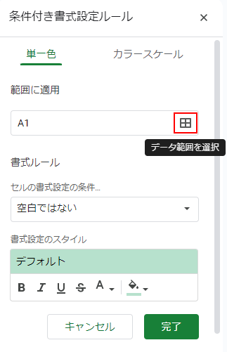
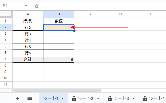
「データ範囲を選択」をクリックします。
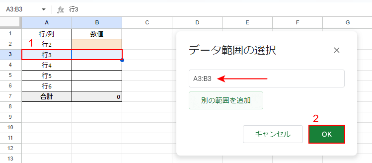
「データ範囲の選択」が表示されます。
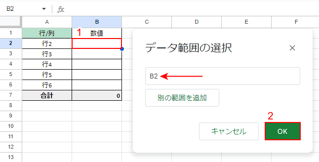
①条件の対象となるセルを選択し、②「OK」ボタンをクリックします。
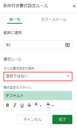
「セルの書式設定の条件…」をクリックします。
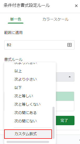
「カスタム数式」を選択します。
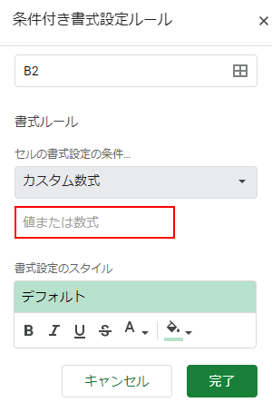
「値または数式」をクリックします。
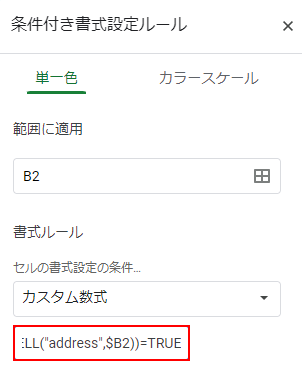
「=INDIRECT("'シート2'!"&CELL("address",$B2))=TRUE」と入力します。
これは「シート2のB2セルを参照し、もしチェックボックスがチェックされていれば」を意味します。
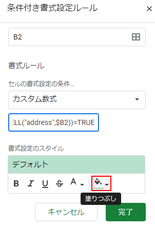
「塗りつぶし」をクリックします。
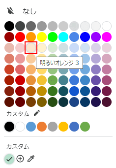
色(例:明るいオレンジ 3)を選択します。
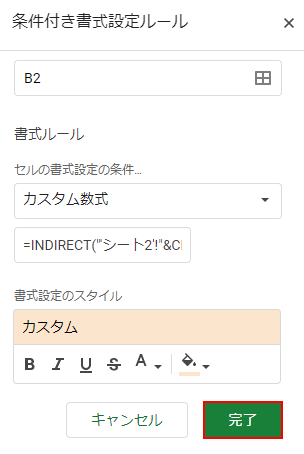
「完了」ボタンをクリックします。
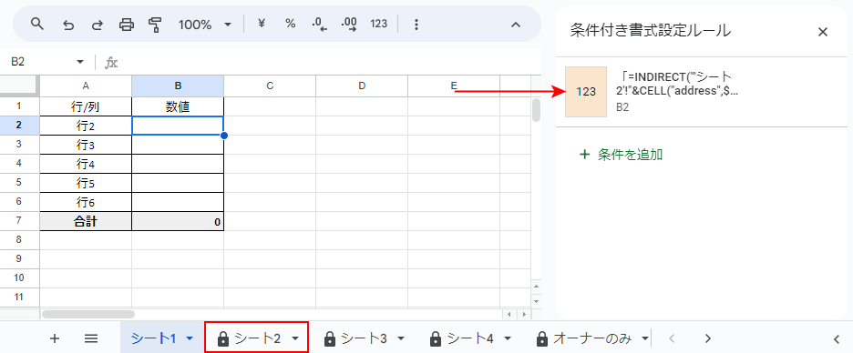
条件付き書式設定ルールが追加されました。
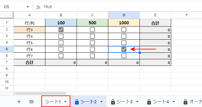
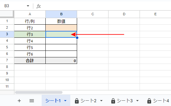
シート2をクリックします。
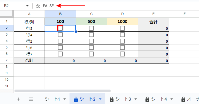
条件としたB2セルはチェックがないのでFALSEと表示されています。
B2セルのチェックボックスをクリックし、チェックを入れます。
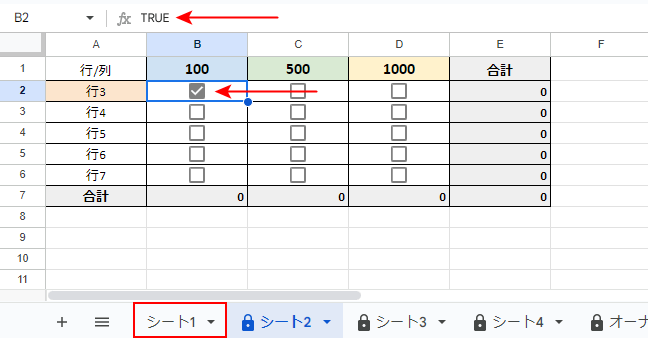
チェックを入れることで、TRUEと表示されました。
シート1をクリックします。
セルの色が変わりました。
これで別シートのセルを参照して条件付き書式を設定できました。
別シートの範囲を条件とする
別シートの範囲にあるセルのいずれかを条件とする場合、COUNTIF関数を併用します。
COUNTIF関数とは、指定した範囲内にあるセルから、特定の条件に当てはまるセルの数をカウントする関数です。
以下より、別シートの範囲にあるセルのいずれかを条件とする設定方法を詳しく解説します。
「データ範囲の選択」を開き、①条件の対象となる範囲を選択し、②「OK」ボタンをクリックします。
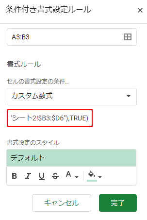
「カスタム数式」に「=COUNTIF(INDIRECT("シート2!$B3:$D6"),TRUE)」と入力します。
これは「シート2のB3からD6の範囲を参照して、もし範囲内のいずれかのチェックボックスがチェックされていたら」を意味します。
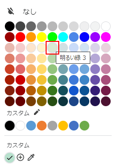
「塗りつぶし」で色(例:明るい緑 3)を選択します。
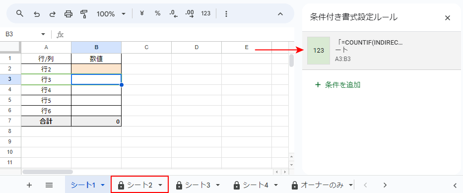
条件付き書式設定ルールが追加されました。
シート2をクリックします。
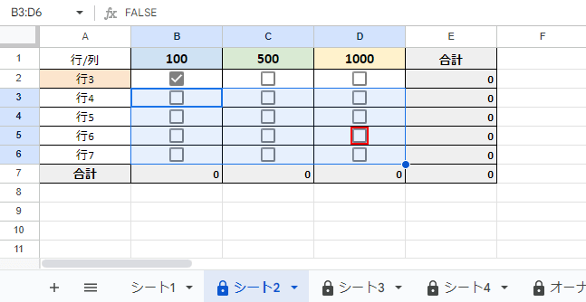
条件とした範囲内のチェックボックスをクリックし、チェックを入れます。
チェックを入れました。
シート1をクリックします。
設定した範囲の色が変わりました。
これで別シートの範囲を参照して条件付き書式を設定できました。